Dielectric Dividing Surface & Box model¶

This example shows how to construct the Dielectric Dividing Surface and the corresponding box model for a confined water system. It starts from precomputed relative permittivity profiles, extracts a bulk dielectric constant from the center of the pore, and then estimates the effective-medium response as outlined in the explanations on Relative permittivity profiles.

import matplotlib.pyplot as plt
import numpy as np
from matplotlib.patches import Rectangle


def draw_effective_box(ax, leff, value, color="C1", label=None):
    """Draw a finite effective-medium slab centered in the pore."""
    xmin, xmax = ax.get_xlim()
    x_center = 0
    rect = Rectangle(
        (x_center - leff / 2, 0),
        leff,
        value,
        facecolor=color,
        edgecolor=color,
        linewidth=2,
        alpha=0.2,
        zorder=4,
        label=label,
    )
    ax.add_patch(rect)

It is important to correctly propagate the errors from the profiles to the effective medium. To this end, we define some helper functions to perform the necessary calculations.

def trapz_err(vals, errs, dx):
    """Integral of a profile with error estimation using the trapezoidal rule."""
    integral = dx / 2 * np.sum(vals[1:] + vals[:-1])
    integral_err = dx / 2 * np.sum(errs[1:] + errs[:-1])
    return integral, integral_err


def bulk_eps(z, eps, err, bulk_dist=15):
    """Estimate the bulk dielectric constant from the pore center."""
    bulk_filter = np.abs(z - 0.5 * (z[0] + z[-1])) < bulk_dist

    if not np.any(bulk_filter):
        return np.nan, np.nan

    weights = 1 / err[bulk_filter] ** 2
    eps_blk = np.average(eps[bulk_filter], weights=weights)
    eps_blk_err = np.sqrt(1 / np.sum(weights))

    return eps_blk, eps_blk_err


def calc_leff_trapz(z, profile, err, length, bulk_response):
    """Calculate the effective length from the profile using the trapezoidal rule."""
    dx = z[1] - z[0]
    integral, integral_err = trapz_err(profile, err, dx)
    leff = (integral - length) / (bulk_response - 1)
    leff_err = integral_err * np.abs(1 / (bulk_response - 1))
    return leff, leff_err


def effective_response(z, profile, err, leff, length, leff_err):
    """Effective-medium response from the profile and the effective length."""
    dx = z[1] - z[0]
    integral, integral_err = trapz_err(profile, err, dx)
    response = 1 + ((integral - length) / leff)
    response_err = integral_err * np.abs(1 / leff) + leff_err * np.abs(
        (integral - length) / leff**2
    )
    return response, response_err

Load the relative permittivity profiles

These files contain the precomputed relative permittivity profile from a simulation of confined water. Here, we use the TIP4P/\(\varepsilon\) model in a graphene slit pore as an example.

base_path = "./tip4p_data/eps_l0d3"
par = np.loadtxt(f"{base_path}_par.dat")
perp = np.loadtxt(f"{base_path}_perp.dat")

The profiles store the dielectric susceptibility, i.e. \(\varepsilon_\parallel - 1\) and \(\varepsilon_\perp^{-1} - 1\), respectively, so we need to add 1 to get the relative permittivity.

z_par, eps_par, eps_par_err = par[:, 0], par[:, 1] + 1, par[:, 2]
z_perp, eps_perp_inv, eps_perp_err = perp[:, 0], perp[:, 1] + 1, perp[:, 2]

Bulk estimate from the pore center

Since the density of the confined water might be different from the bulk density, we cannot simply use the bulk dielectric constant of the water model. Instead, we estimate the bulk dielectric constant from the center of the pore, as described in the documentation.

eps_bulk, eps_bulk_err = bulk_eps(z_par, eps_par, eps_par_err)
print(f"Estimated bulk dielectric constant: {eps_bulk:.2f} ± {eps_bulk_err:.2f}")

Estimated bulk dielectric constant: 76.69 ± 0.02

Indeed, the estimated bulk dielectric constant is close to the known bulk value for the TIP4P/\(\varepsilon\) model, which is around 78.3 at room temperature.

Parallel component

We can now use the estimated bulk dielectric constant to calculate the effective length and effective dielectric constant for the parallel component.

leff_par, leff_par_err = calc_leff_trapz(
    z_par, eps_par, eps_par_err, z_par[-1] - z_par[0], eps_bulk
)
eps_eff_par, eps_eff_par_err = effective_response(
    z_par, eps_par, eps_par_err, leff_par, z_par[-1] - z_par[0], leff_par_err
)

Perpendicular component

The perpendicular profile is stored as \(\varepsilon^{-1}(z)\).

leff_perp, leff_perp_err = calc_leff_trapz(
    z_perp, eps_perp_inv, eps_perp_err, z_perp[-1] - z_perp[0], 1 / eps_bulk
)
eps_eff_perp_inv, eps_eff_perp_inv_err = effective_response(
    z_perp, eps_perp_inv, eps_perp_err, leff_perp, z_perp[-1] - z_perp[0], leff_perp_err
)
print(f"Effective length (parallel): {leff_par:.2f} ± {leff_par_err:.2f}")
print(f"Effective length (perpendicular): {leff_perp:.2f} ± {leff_perp_err:.2f}")

Effective length (parallel): 60.03 ± 0.12
Effective length (perpendicular): 56.90 ± 1.55

We see that the effective length differs for the parallel and perpendicular components. For the graphene interface studied here, the confined system screens electrostatic interactions more efficiently than a bulk-like system of the same slab thickness, thus the effective length is larger than the physical slab thickness. [1]

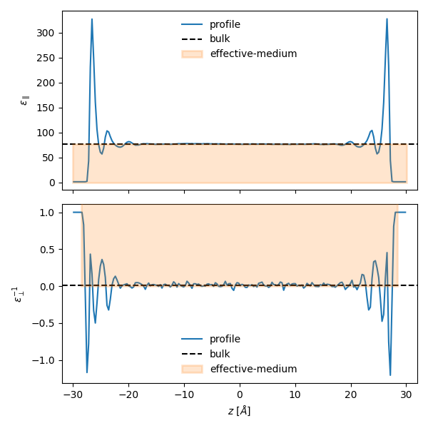
Plot the raw profiles together with the effective-medium estimate

fig, ax = plt.subplots(2, sharex=True, figsize=(6, 6))

ax[0].set_xlim(-32, 32)
ax[1].set_xlim(-32, 32)

ax[0].plot(z_par, eps_par, label="profile")
ax[0].axhline(eps_bulk, color="black", linestyle="dashed", label="bulk")
ax[0].set_ylabel(r"$\varepsilon_{\parallel}$")
draw_effective_box(ax[0], leff_par, eps_eff_par, label="effective-medium")
ax[0].legend(frameon=False)

ax[1].plot(z_perp, eps_perp_inv, label="profile")
ax[1].axhline(1 / eps_bulk, color="black", linestyle="dashed", label="bulk")
ax[1].set_xlabel(r"$z$ [$\AA$]")
ax[1].set_ylabel(r"$\varepsilon_{\perp}^{-1}$")
draw_effective_box(ax[1], leff_perp, 1 / eps_eff_perp_inv, label="effective-medium")
ax[1].legend(frameon=False)

fig.tight_layout()
plt.show()

References¶

Gallery generated by Sphinx-Gallery