Dielectric profile calculation

Basic usage

In the following example, we will show how to calculate the dielectric profiles as described in Dielectric constant measurement.

Before producing trajectories to calculate dielectric profiles, you will need to consider which information you will need and thus need to print out. The dielectric profile calculators need unwrapped positions and charges of all charged atoms in the system. Unwrapped refers to the fact that you will need either “repaired” molecules (which in GROMACS trjconv with the -pbc mol option can do for you) or you will need to provide topology information for MAICoS to repair molecules for you during the analysis. Note, however, that unwrapping adds overhead to your calculations. Therefore, it is recommended to use a repaired trajectory if possible.

In the following, we will give an example of a trajectory of water confined by graphene sheets simulated via GROMACS. We assume that the GROMACS topology is given by graphene_water.tpr and the trajectory is given by graphene_water.xtc. Both can be downloaded under topology and trajectory, respectively.

From these files you can create a MDAnalysis universe object.

import matplotlib.pyplot as plt
import MDAnalysis as mda
import numpy as np

import maicos


u = mda.Universe("graphene_water.tpr", "graphene_water.xtc")

This universe object can then be passed to the dielectric profile analysis object, documented in maicos.DielectricPlanar. It expects you to pass the atom groups you want to perform the analysis for. In our example, we have graphene walls and SPC/E water confined between them, where we are interested in the dielectric behavior of the fluid. Thus, we will first select the water as an MDAnalysis atom group using MDAnalysis.core.groups.AtomGroup.select_atoms(). In this case we select the water by filtering for the residue named SOL.

According to the discussion above, we use an unwrapped trajectory and set the unwrap = False keyword.

The simulation trajectory that we provide was simulated using Yeh-Berkowitz dipole correction. So we don’t want to include dipole corrections, because we assume that our simulation data adequately represents a 2d-periodic system. For systems that are not 2d-periodic, one should set the is_3d argument to True to include the dipole correction (see Dielectric constant measurement or the section on boundary conditions down below).

Since we included a large vacuum region in our simulation that is not of interest for the dielectric profile, we can set the refgroup to the group containing our water molecules. This will calculate the dielectric profile relative to the center of mass of the water in the region of interest.

water = u.select_atoms("resname SOL")
# Create the analysis object with the appropriate parameters.
analysis_obj = maicos.DielectricPlanar(water, bin_width=0.1, refgroup=water)

This creates the analysis object, but does not yet perform the analysis. To this end we call the member function run. We may set the verbose keyword to True to get additional information like a progress bar.

Here you also have the chance to set start and stop keywords to specify which frames the analysis should start at and where to end. One can also specify a step keyword to only analyze every step frames.

analysis_obj.run(step=5)

/home/docs/checkouts/readthedocs.org/user_builds/maicos/envs/main/lib/python3.9/site-packages/maicos/core/base.py:456: UserWarning: Your data seems to be correlated with a correlation time which is 2.55 times larger than your step size. Consider increasing your step size by a factor of 5 to get a reasonable error estimate.
  self.corrtime = correlation_analysis(self.timeseries)

<maicos.modules.dielectricplanar.DielectricPlanar object at 0x7fad79bdfe50>

Here we use step = 5 to run a fast analysis. You may reduce the step parameter to gain a higher accuracy. Note that the analysis issues a warning concerning the correlation time of the trajectory, which is automatically calculated as an indication of how far apart the frames should be chosen to get a statistically uncertainty indicator estimate. For small trajectories such as the one in this example, this estimate is not very reliable and one should perform the analysis for longer trajectories for actual production runs.

Hence, we will ignore the warning for the purpose of this example. Now we are ready to plot the results. MAICoS provides the outcome of the calculation as sub-attributes of the results attribute of the analysis object. The results object contains several attributes that can be accessed directly. For example, the bin positions are stored in the bin_pos attribute, the parallel and perpendicular dielectric profiles in the eps_par and eps_perp attributes respectively. (See maicos.DielectricPlanar for a full list of attributes.)

For this example, we plot both profiles using matplotlib. Note that MAICoS always centers the system at the origin or the selected refgroup, so here we set the limits of the x-axis to [-7, 7]. Then we can only show the relevant part of the output (the system has a width of 14 Å).

fig, ax = plt.subplots(2, sharex=True)

z = analysis_obj.results.bin_pos

ax[0].plot(z, analysis_obj.results.eps_perp)
ax[1].plot(z, analysis_obj.results.eps_par)

ax[0].set_ylabel(r"$\varepsilon^{-1}_{\perp} - 1$")
ax[1].set_ylabel(r"$\varepsilon_{\parallel} - 1$")

ax[1].set_xlabel(r"$z$")

# Only plot the actual physical system:
ax[0].set_xlim([-7, 7])
ax[1].set_xlim([-7, 7])

# Also plot the bulk values for reference
ax[0].axhline(1 / 71 - 1, color="black", linestyle="dashed")
ax[1].axhline(71 - 1, color="black", linestyle="dashed")

fig.tight_layout()
plt.show()

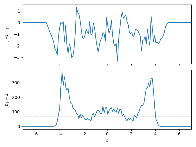
A few notes on the results: The perpendicular component is given as the inverse of the dielectric profile, which is the “natural” output (see Dielectric constant measurement for more details). Furthermore, the bulk values expected for the SPC/E water model are given as reference lines.

Notice that the parallel component is better converged than the perpendicular component which in this very short trajectory is still noisy. For trajectories with a duration of about 1 microsecond, the perpendicular component can be expected to be converged.

Boundary Conditions

(See Dielectric constant measurement for a thorough discussion of the boundary conditions). Here we only note that the is_3d flag has to be chosen carefully, depending on if one simulated a truly 3d periodic system or a 2d periodic one. Seldomly, vacuum boundary conditions might have been used for Ewald summations instead of the more common tin-foil boundary conditions. In this case, the vac flag should be set to True.

TIP4P Water and Molecules with Virtual Sites

One has to be careful when using the dielectric profile analysis for systems with virtual sites, such as TIP4P water. The reason is that the virtual sites might not be included in the trajectory, but instead are only constructed by the MD engine during the force calculation. (For example some LAMMPS fixes)

This problem can be circumvented by creating the virtual sites by hand. This is done by creating a transformation function that is added to the universe. This function is called for every frame and can be used to create the virtual sites. The following example shows how to do this for TIP4P/ε water from a LAMMPS trajectory. Here we only shift the oxygen charge along the H-O-H angle bisector by a distance of 0.105 Å, which is the distance between the oxygen charge and the virtual site in the TIP4P/ε water model.

def transform_lammps_tip4p(
    oxygen_index_array: np.ndarray, distance: float
) -> mda.coordinates.timestep.Timestep:
    """Creates a transformation function where for lammps tip4p molecukes.

    oxygen_index_array is the array of indices where ``atom.type == oxygen_type``.
    I.e. given by ``np.where(universe.atoms.types == oxygen_type)[0]``.

    ``distance`` defines by how much the oxygen is moved in the H-O-H plane.
    """

    def wrapped(timestep):
        # shift oxygen charge in case of tip4p
        this_pos = timestep.positions
        for j in oxygen_index_array:
            # -2 * vec_o + vec_h1 + vec_h2
            vec = np.dot(np.array([-2, 1, 1]), this_pos[j : j + 3, :])
            unit_vec = vec / np.linalg.norm(vec)
            this_pos[j] += unit_vec * distance
        return timestep

    return wrapped


oxygen_index_array = u.select_atoms("type 2").indices

shift_tip4p_lammps = transform_lammps_tip4p(oxygen_index_array, 0.105)

u.trajectory.add_transformations(shift_tip4p_lammps)

Preliminary Output

As the dielectric analysis is usually run for long trajectories, analysis can take a while. Hence, it is useful to get some preliminary output to see how the analysis is progressing. Use the concfreq keyword to specify how often the analysis should output the current results into data files on the disk. The concfreq keyword is given in units of frames. For example, if concfreq = 100, the analysis will output the current results to the data files every 100 frames.