Small-angle X-ray scattering

Small-angle X-ray scattering (SAXS) can be extracted using MAICoS. To follow this how-to guide, you should download the topology and the trajectory files of the water system.

For more details on the theory see Small-angle X-ray scattering.

First, we import Matplotlib, MDAnalysis, NumPy and MAICoS:

import matplotlib.pyplot as plt
import MDAnalysis as mda
from MDAnalysis.analysis.rdf import InterRDF

import maicos
from maicos.lib.math import compute_form_factor, compute_rdf_structure_factor

The water system consists of 510 water molecules in the liquid state. The molecules are placed in a periodic cubic cell with an extent of \(25 \times 25 \times 25\,\textrm{Å}^3\).

Load Simulation Data

Create a MDAnalysis.core.universe.Universe and define a group containing only the oxygen atoms and a group containing only the hydrogen atoms:

u = mda.Universe("water.tpr", "water.trr")

group_O = u.select_atoms("type O*")
group_H = u.select_atoms("type H*")

Extract small angle x-ray scattering (SAXS) intensities

Let us use the maicos.Saxs class of MAICoS and apply it to all atoms in the system:

saxs = maicos.Saxs(u.atoms).run(stop=30)

Note

SAXS computations are extensive calculations. Here, to get an overview of the scattering intensities, we reduce the number of frames to be analyzed from 101 to 30, by adding the stop = 30 parameter to the run method. Due to the small number of analyzed frames, the scattering intensities shown in this tutorial should not be used to draw any conclusions from the data.

Extract the scattering vectors and the averaged structure factor and SAXS scattering intensities from the results attribute:

scattering_values = saxs.results.scattering_vectors
structure_factors = saxs.results.structure_factors
scattering_intensities = saxs.results.scattering_intensities

The scattering intensities (and structure factors) are given as a 1D array, let us look at the 10 first lines:

print(scattering_intensities[:10])

[1.62620077 0.91205581 1.32501428 1.75529088 1.20605233 2.13058505
 2.14645164 2.39313797 2.74842731 3.34680856]

By default, the binwidth in the recipocal \((q)\) space is \(0.1 Å^{-1}\).

We now plot the structure factor as well a the scattering intensities together.

fig1, ax1 = plt.subplots(nrows=2, sharex=True, layout="constrained")

ax1[0].plot(scattering_values, structure_factors)
ax1[1].plot(scattering_values, scattering_intensities)

ax1[-1].set_xlabel(r"q (1/Å)")

ax1[0].set_ylabel(r"structure factor $S(q)$")
ax1[1].set_ylabel(r"scattering intensities $I(q)$")
fig1.align_labels()

fig1.show()

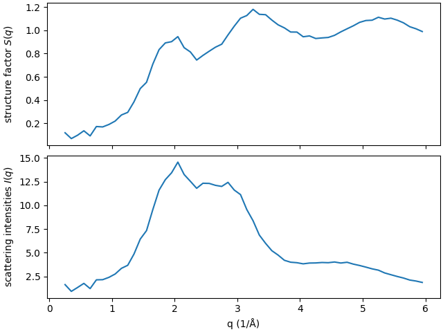
The structure factor \(S(q)\) and the scattering intensities \(I(q)\) are related via

\[I(q) = [f(q)]^2 S(q)\]

where \(f(q)\) are the atomic form factors. We will investigate the relation below in more details.

Computing oxygen and hydrogen contributions

An advantage of full atomistic simulations is their ability to investigate atomic contributions individually. Let us calculate both oxygen and hydrogen contributions, respectively:

saxs_O = maicos.Saxs(group_O).run(stop=30)
saxs_H = maicos.Saxs(group_H).run(stop=30)

Let us plot the results for the structure factor, the squared form factor as well scattering intensities together. For computing the form factor we will use maicos.lib.math.compute_form_factor(). Note that here we access the results directly from the results attribute without storing them in individual variables before:

fig2, ax2 = plt.subplots(nrows=3, sharex=True, layout="constrained")

# structure factors
ax2[0].plot(
    saxs_O.results.scattering_vectors,
    saxs_O.results.structure_factors,
    label="Oxygen",
)
ax2[0].plot(
    saxs_H.results.scattering_vectors,
    saxs_H.results.structure_factors,
    label="Hydrogen",
)

# form factors
ax2[1].plot(
    saxs_O.results.scattering_vectors,
    compute_form_factor(saxs_O.results.scattering_vectors, "O") ** 2,
)
ax2[1].plot(
    saxs_H.results.scattering_vectors,
    compute_form_factor(saxs_H.results.scattering_vectors, "H") ** 2,
)

# scattering intensitie
ax2[2].plot(saxs_O.results.scattering_vectors, saxs_O.results.scattering_intensities)
ax2[2].plot(saxs_H.results.scattering_vectors, saxs_H.results.scattering_intensities)

ax2[-1].set_xlabel(r"q (1/Å)")
ax2[0].set_ylabel(r"$S(q)$")
ax2[1].set_ylabel(r"$f(q)^2$")
ax2[2].set_ylabel(r"$I(q)$")

ax2[0].legend()
fig2.align_labels()

fig2.show()

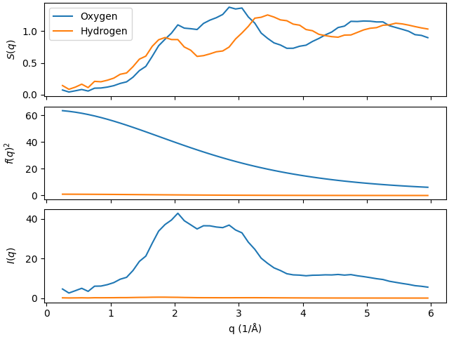
The figure above nicely shows that multiplying the structure factor \(S(q)\) and the squared form factor \(f(q)^2\) results in the scattering intensity \(I(q)\). Also, it is worth to notice that due to small form factor of hydrogen there is basically no contribution of the hydrogen atoms to the total scattering intensity of water.

Connection of the structure factor to the radial distribution function

As in details explained in Small-angle X-ray scattering, the structure factor can be related to the radial distribution function (RDF). We denote this structure factor by \(S^\mathrm{FT}(q)\) since it is based on Fourier transforming the RDF. The structure factor which can be directly obtained from the trajectory is denoted by \(S^\mathrm{D}(q)\).

To relate these two we first calculate the oxygen-oxygen RDF up to half the box length using MDAnalysis.analysis.rdf.InterRDF and save the result in variables for an easier access.

box_lengh = u.dimensions[0]

oo_inter_rdf = InterRDF(
    g1=group_O, g2=group_O, range=(0, box_lengh / 2), exclude_same="residue"
).run()

r_oo = oo_inter_rdf.results.bins
rdf_oo = oo_inter_rdf.results.rdf

We use exclude_same="residue" to exclude atomic self contributions resulting in a large peak at 0. Next, we convert the RDF into a structure factor using maicos.lib.math.compute_rdf_structure_factor() and the number density of the oxygens.

density = group_O.n_atoms / u.trajectory.ts.volume

q_rdf, struct_factor_rdf = compute_rdf_structure_factor(
    rdf=rdf_oo, r=r_oo, density=density
)

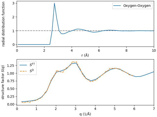
Now we can plot everything together and find that the direct evaluation from above and the transformed RDF give the same structure factor.

fig3, ax3 = plt.subplots(2, layout="constrained")

ax3[0].axhline(1, c="gray", ls="dashed")
ax3[0].plot(r_oo, rdf_oo, label="Oxygen-Oxygen")
ax3[0].set_xlabel("r (Å)")
ax3[0].set_ylabel("radial distribution function")
ax3[0].set_xlim(0, 10)

ax3[1].plot(q_rdf, struct_factor_rdf, label=r"$S^\mathrm{FT}$")
ax3[1].plot(
    saxs_O.results.scattering_vectors,
    saxs_O.results.structure_factors,
    label=r"$S^\mathrm{D}$",
    ls="dashed",
)

ax3[1].set_xlabel("q (1/Å)")
ax3[1].set_ylabel("structure factor $S(q)$")
ax3[1].set_xlim(0, 7)

ax3[1].legend()
ax3[0].legend()
fig3.align_labels()

fig3.show()