Small-angle X-ray scattering#
MD Simulations often complement conventional experiments, such as X-ray crystallography, Nuclear Magnetic Resonance (NMR) spectroscopy and Atomic-Force Microscopy (AFM). X-ray crystallography is a method by which the structure of molecules can be resolved. X-rays of wavelength 0.1 to 100 Å are scattered by the electrons of atoms. The intensities of the scattered rays are often amplified using by crystals containing a multitude of the studied molecule positionally ordered. The molecule is thereby no longer under physiological conditions. However, the study of structures in a solvent should be done under physiological conditions (in essence, this implies a disordered, solvated fluid system); therefore X-ray crystallography does not represent the ideal method for such systems. Small-Angle X-ray Scattering (abbreviated to SAXS) allows for measurements of molecules in solutions. With this method the shape and size of the molecule and also distances within it can be obtained. In general, for larger objects, the information provided by SAXS can be converted to information about the object’s geometry via the Bragg-Equation
with \(n \in \mathbb{N}\), \(\lambda\) the wavelength of the incident wave, \(d\) the size of the diffracting object, and \(\theta\) the scattering angle. For small angles, \(d\) and \(\theta\) are approximately inversely proportional to each other, which means larger objects scatter X-rays at smaller angles.
Experiments#
The measured quantity in SAXS experiments is the number of elastically scattered photons as a function of the scattering angle \(2\theta\), i.e. the intensity of the scattered rays across a range of small angles. The general set-up of a SAXS experiment is shown in figure below.
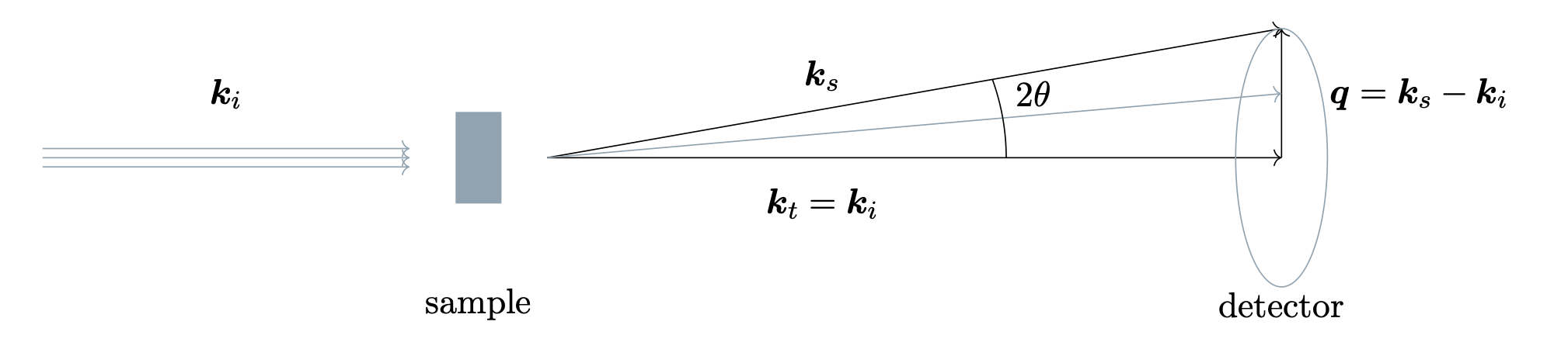
The experiments are carried out by placing the sample of interest in a highly monochromatic and collimated (parallel) X-ray beam of wavelength \(\lambda\). When the incident rays with wave vector \(\boldsymbol{k}_i\) reach the sample they scatter. The scattered rays, with wave vector \(\boldsymbol{k}_s\), are recorded by a 2D-detector revealing a diffraction pattern.
Since the scattering agents in the sample are electrons, X-Ray diffraction patterns reveal the electron density. Since the scattering is elastic, the magnitudes of the incident and scattered waves are the same: \(|\boldsymbol{k}_i| = |\boldsymbol{k}_s| = 2\pi/\lambda\). The scattering vector is \(\boldsymbol{q} = \boldsymbol{k}_s - \boldsymbol{k}_i\) with a magnitude of \(q = |\boldsymbol{q}| = 4\pi \sin(\theta)/\lambda\). The structure factor can be obtained from the intensity of the scattered wave, \(I_s(\boldsymbol{q})\), and the correspnding form factor \(f (q)\), which involves a frourier transform of the element-specific local electron density and thus determines the amplitude of the scattered wave of a single element.
Simulations#
In simulations, the structure factor and scattering intensities
\(S(\boldsymbol{q})\) can be extracted directly from the positions of the particles.
maicos.Saxs calculates these factors. The calculated scattering intensities can
be directly compared to the experimental one without any further processing. In the
following we derive the essential relations. We start with the scattering intensity
which is expressed as
with the amplitude of the elastically scattered wave
where \(f_j(q)\) is the element-specific form factor of atom \(j\) and \(\boldsymbol{r}_j\) the position of the \(j\) th atom out of \(N\) atoms.
The scattering intensity can be evaluated for wave vectors \(\boldsymbol q = 2 \pi (L_x n_x, L_y n_y, L_z n_z)\), where \(n \in \mathbb N\) and \(L_x, L_y, L_z\) are the box lengths of cubic cells.
Note
maicos.Saxs can analyze any cells by mapping coordinates back onto cubic
cells.
The complex conjugate of the amplitude is
The scattering intensity therefore can be written as
With Euler’s formula \(e^{i\phi} = \cos(\phi) + i \sin(\phi)\) the intensity is
Multiplication of the terms and simplifying yields the final expression for the intensity of a scattered wave as a function of the wave vector and with respect to the particle’s form factor
For systems containing only one kind of atom the structure factor is connected to the scattering intensity via
For any system the structure factor can be written as
The limiting value \(S(0)\) for \(q \rightarrow 0\) is connected to the isothermal compressibility [1] and the element-specific form factors \(f(q)\) of a specific atom can be approximated with
Expressed in terms of the scattering vector we can write
The element-specific coefficients \(a_{1,\dots,4}\), \(b_{1,\dots,4}\) and \(c\) are documented [2].
Connection of the structure factor to the radial distribution function#
If the system’s structure is determined by pairwise interactions only, the density correlations of a fluid are characterized by the pair distribution function
where \(\rho^{(2)}(\boldsymbol r, \boldsymbol r\prime) = \sum_{i,j=1, i\neq j}^{N} \delta (\boldsymbol r - \boldsymbol r_i) \delta (\boldsymbol r - \boldsymbol r_j)\) and \(\rho(\boldsymbol r) = \sum_{i=1}^{N} \delta (\boldsymbol r - \boldsymbol r_i)\) are the two- and one-particle density operators.
For a homogeneous and isotropic system, \(g(r) = g(\boldsymbol r, \boldsymbol r^\prime)\) is a function of the distance \(r =|\boldsymbol r - \boldsymbol r^\prime|\) only and is called the radial distribution function (RDF). As explained above, scattering experiments measure the structure factor
which we here normalize only by the number of particles \(N\). For a homogeneous and isotropic system, it is a function of \(q = |\boldsymbol q|\) only and related to the RDF by Fourier transformation (FT)
which is another way compared for the direct evaluation from trajectories which was derived above. In general this can be as accurate as the direct evaluation if the RDF implementation works for non-cubic cells and is not limited to distances \(r_\mathrm{max} = L/2\), see [3] for details. However, in usual implementation the RDF can only be obtained until \(r_\mathrm{max} = L/2\) which leads to a range of \(q > q_\mathrm{min}^\mathrm{FT} = 2\pi / r_\mathrm{rmax} = 4 \pi /L\). This means that the minimal wave vector that can be resolved is a factor of 2 larger compared compared to the direct evaluation, leading to “cutoff ripples”. The direct evaluation should therefore usually be preferred [4].
To compare the RDF and the structure factor you can use
maicos.lib.math.compute_rdf_structure_factor(). For a detailed example take
a look at Small-angle X-ray scattering.