Calculating and interpreting dipolar pair correlation functions

In this examples we will calculate dipolar pair correlation functions in real and Fourier space using the maicos modules maicos.RDFDiporder and maicos.DiporderStructureFactor. We will show how these pair correlation functions are connected to each other and electrostatic properties like the dielectric constant \(\varepsilon\) and the Kirkwood factor \(g_K\).

We start by importing the necessarary modules

import matplotlib.pyplot as plt
import MDAnalysis as mda
import numpy as np
import scipy
from MDAnalysis.analysis.dielectric import DielectricConstant

import maicos
from maicos.lib.math import compute_rdf_structure_factor

Our example system is \(N=512\) rigid SPC/E water molecules simulated in an NVT ensemble at \(300\,\mathrm{K}\) in a cubic cell of \(L=24.635\,Å\). To follow this how-to guide, you should download the topology and the trajectory files of the system. Below we load the system, report and store some system properties for later usage.

u = mda.Universe("water_nvt.tpr", "water_nvt.xtc")

volume = u.trajectory.ts.volume
density = u.residues.n_residues / volume
dipole_moment = u.atoms.dipole_moment(compound="residues", unwrap=True).mean()

print(f"ρ_n = {density:.3f} Å^-3")
print(f"µ = {dipole_moment:.2f} eÅ")

ρ_n = 0.034 Å^-3
µ = 0.49 eÅ

The results of our first property calculations show that the number density as well as the dipole moment of a single water molecule is consistent with the literature [1].

Static dielectric constant

To start with the analysis we first look at the dielectric constant of the system. If you run a simulation using an Ewald simulation technique as usually done, the dielectric constant for such system with metallic boundary conditions is given according to Neumann[2] by

\[\varepsilon = 1 + \frac{\langle M^2 \rangle_\mathrm{MBE} - \langle M \rangle_\mathrm{MBE}^2}{3 \varepsilon_0 V k_B T}\]

where

\[\boldsymbol M = \sum_{i=1}^N \boldsymbol \mu_i\]

is the total dipole moment of the box, \(V\) its volume and \(\varepsilon_0\) the vacuum permittivity. We use the subscript in the expectation value \(\mathrm{MBE}\) indicating that the equation only holds for simulations with Metallic Boundary conditions in an Ewald simulation style. As shown in the equation for \(\varepsilon(\mathrm{MBE})\) the dielectric constant here is a total cell quantity connecting the fluctuations of the total dipole moment to the dielectric constant. We can calculate \(\varepsilon_\mathrm{MBE}\) using the MDAnalysis.analysis.dielectric.DielectricConstant module of MDAnalysis.

epsilon_mbe = DielectricConstant(atomgroup=u.atoms).run()
print(f"ɛ_MBE = {epsilon_mbe.results.eps_mean:.2f}")

ɛ_MBE = 69.21

The value of 70 is the same as reported in the literature for the rigid SPC/E water model [1].

Kirkwood factor

Knowing the dielectric constant we can also calculate the Kirkwood factor \(g_K\) which is a measure describing molecular correlations. I.e a Kirkwood factor greater than 1 indicates that neighboring molecular dipoles are more likely to align in the same direction, enhancing the material’s polarization and, consequently, its dielectric constant. Based on the dielectric constant \(\varepsilon\) Kirkwood and Fröhlich derived the relation for the factor \(g_K\) according to

\[\frac{ N \mu^2 g_K}{\varepsilon_0 V k_B T} = \frac{(\varepsilon - 1)(2\varepsilon + 1)}{\varepsilon}\]

This relation is valid for a sample in an infinity, homogenous medium of the same dielectric constant. Below we implement this equation and calculate the factor for our system.

def kirkwood_factor_KF(
    dielectric_constant: float,
    volume: float,
    n_dipoles: float,
    molecular_dipole_moment: float,
    temperature: float = 300,
) -> float:
    """Kirkwood factor in the Kirkwood-Fröhlich way.

    For the sample in an infinity, homogenous medium of the same dielectric constant.

    Parameters
    ----------
    dielectric_constant : float
        the static dielectric constant ɛ
    volume : float
        system volume in Å^3
    n_dipoles : float
        number of dipoles
    molecular_dipole_moment : float
        dipole moment of a molecule (eÅ)
    temperature : float
        temperature of the simulation K
    """
    dipole_moment_sq = (
        molecular_dipole_moment
        * scipy.constants.elementary_charge
        * scipy.constants.angstrom
    ) ** 2
    factor = (
        scipy.constants.epsilon_0
        * (volume * scipy.constants.angstrom**3)
        * scipy.constants.Boltzmann
        * temperature
    )

    return (
        factor
        / (dielectric_constant * n_dipoles * dipole_moment_sq)
        * (dielectric_constant - 1)
        * (2 * dielectric_constant + 1)
    )


kirkwood_KF = kirkwood_factor_KF(
    dielectric_constant=epsilon_mbe.results.eps_mean,
    volume=volume,
    n_dipoles=u.residues.n_residues,
    molecular_dipole_moment=dipole_moment,
)

print(f"g_K = {kirkwood_KF:.2f}")

g_K = 2.39

This value means there is a quite strong correlation between neighboring water molecules. The dielectric constant \(\varepsilon\) is a material property and does not depend on the boundary condition. Instead, the Kirkwood factor is indicative of dipole-dipole correlations which instead depend on the boundary condistions in the simulation. This relation is described and shown below.

Connecting the Kirkwood factor to real space dipolar pair-correlation functions

The \(r\)-dependent Kirkwood factor can also be calculated from real space dipole-dipole pair correlation function [3]

\[g_\mathrm{\hat{\boldsymbol{\mu}}, \hat{\boldsymbol{\mu}}}(r) = \frac{1}{N} \left\langle \sum_i \frac{1}{n_i(r)} \sum_{j=1}^{n_i(r)} (\hat{\boldsymbol{\mu}}_i \cdot \hat{\boldsymbol{\mu}}_j) \right \rangle\]

where \(\hat{\boldsymbol{\mu}}\) is the normalized dipole moment and \(n_i(r)\) is the number of dipoles within a spherical shell of distance \(r\) and \(r + \delta r\) from dipole \(i\). We compute the pair correlation function using the maicos.RDFDiporder module up to half of the length of cubic simulation box. We drop a delta like contribution in \(r=0\) caused by interaction of the dipole with itself.

L_half = u.dimensions[:3].max() / 2

rdf_diporder = maicos.RDFDiporder(g1=u.atoms, rmax=L_half, bin_width=0.01)
rdf_diporder.run()

<maicos.modules.rdfdiporder.RDFDiporder object at 0x7fad78d82fa0>

Based on this correlation function we can calculate the radially resolved Kirkwood factor via [4]

\[G_K(r) = \rho_n 4 \pi \int_0^r \mathrm{d}r^\prime {r^\prime}^2 g_\mathrm{\hat \mu, \hat \mu}(r^\prime) + 1\]

where the “\(+ 1\)” accounts for the integration of the delta function at \(r=0\). Here \(\rho_n = N/V\) is the density of dipoles.

radial_kirkwood = 1 + (
    density
    * 4
    * np.pi
    * scipy.integrate.cumulative_trapezoid(
        x=rdf_diporder.results.bins,
        y=rdf_diporder.results.bins**2 * rdf_diporder.results.rdf,
        initial=0,
    )
)

While, for a truly infinite system, the \(r\)- dependent Kirkwood factor, \(G_\mathrm{K}(r)\) is short range [5] [4], the boundary conditions on a finite system introduce long-range effects. In particular, within MBE, Caillol[6] has shown that \(G_\mathrm{K}(r)\) has a spurious asymptotic growth proportional to \(r^3/V\). This effect is stil present at \(r=r_K\), where \(r_K\) (here approximately 6 Å) indicates a distance after which all the physical features of \(g_\mathrm{\hat{\boldsymbol{\mu}},\hat{\boldsymbol{\mu}}}(r)\) are extinct. For more details see the original literature. Below we show the pair correlation function as well as the radial and the (static) Kirkwood factor as gray dashed line.

fig, ax = plt.subplots(2)

ax[0].plot(
    rdf_diporder.results.bins,
    rdf_diporder.results.rdf,
)
ax[1].axhline(kirkwood_KF, ls="--", c="gray", label="$g_K$ (KF)")

ax[1].plot(rdf_diporder.results.bins, radial_kirkwood)

ax[0].set(
    xlim=(2, 6),
    ylim=(-0.2, 1.5),
    ylabel=r"$g_\mathrm{\hat{\boldsymbol{\mu}}, \hat{\boldsymbol{\mu}}}(r)$",
)

ax[1].set(
    xlim=(2, 10),
    ylim=(0.95, 3.9),
    xlabel=r"$r\,/\,\mathrm{Å}$",
    ylabel=r"$G_K(r)$",
)

ax[1].legend()

fig.align_labels()
fig.tight_layout()

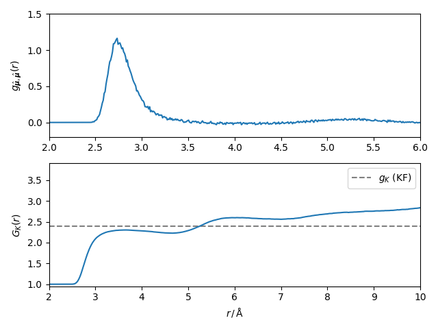
Notice that the Kirkwood Fröhlich estimator for the Kirkwood factors differs from the value of \(G_K(r=r_K)\) obtained from simulations in the MBE ensemble.

Dipole Structure factor

An alternative approach to calculate the dielectric constant is via the dipole structure factor which is given by

\[S(q)_{\hat{\boldsymbol{\mu}} \hat{\boldsymbol{\mu}}} = \left \langle \frac{1}{N} \sum_{i,j=1}^N \hat \mu_i \hat \mu_j \, \exp(-i\boldsymbol q\cdot [\boldsymbol r_i - \boldsymbol r_j]) \right \rangle\]

We compute the structure factor using the maicos.DiporderStructureFactor module.

diporder_structure_factors = maicos.DiporderStructureFactor(atomgroup=u.atoms, dq=0.05)
diporder_structure_factors.run()

<maicos.modules.diporderstructurefactor.DiporderStructureFactor object at 0x7fad78f6e2b0>

As also shown how to on SAXS calculations the structure factor can also be obtained directly from the real space correlation functions using Fourier transformation via

\[S_{\hat{\boldsymbol{\mu}} \hat{\boldsymbol{\mu}}}^\mathrm{FT}(q) = 1 + 4 \pi \rho \int_0^\infty \mathrm{d}r r \frac{\sin(qr)}{q} g_{\hat \mu\hat \mu}(r)\,,\]

which can be obtained by the function maicos.lib.math.compute_rdf_structure_factor(). We have assumed an isotropic system so that \(S(\boldsymbol q) = S(q)\). Note that we added a one to the dipole pair correlation function due to the implementation of the Fourier transformation inside maicos.lib.math.compute_rdf_structure_factor().

q_rdf, struct_fac_rdf = compute_rdf_structure_factor(
    rdf=1 + rdf_diporder.results.rdf, r=rdf_diporder.results.bins, density=density
)

Before we plot the structure factors we first also fit the low \(q\) limit according to a quadratic function as

\[S_\mathrm{\hat \mu\hat \mu}(q\rightarrow0) \approx S_0 + S_2q^2\]

The fit contains no linear term because of the structure factors’ symmetry around 0.

n_max = 5  # take `n_max` first data points of the structure factor for the fit

# q_max is the maximal q value corresponding to the last point taken for the fit
q_max = diporder_structure_factors.results.scattering_vectors[n_max]
print(f"q_max = {q_max:.2f} Å")

eps_fit = np.polynomial.Polynomial.fit(
    x=diporder_structure_factors.results.scattering_vectors[:n_max],
    y=diporder_structure_factors.results.structure_factors[:n_max],
    deg=(0, 2),
    domain=(-q_max, q_max),
)

print(
    f"Best fit parameters: S_0 = {eps_fit.coef[0]:.2f}, S_2 = {eps_fit.coef[2]:.2f} Å^2"
)

q_max = 0.63 Å
Best fit parameters: S_0 = 2.45, S_2 = -0.84 Å^2

Now we can finally plot the structure factor

plt.plot(
    diporder_structure_factors.results.scattering_vectors,
    diporder_structure_factors.results.structure_factors,
    label=r"$S_{\hat \mu\hat \mu}$",
)
plt.plot(
    q_rdf, struct_fac_rdf, ls="dashed", label=r"$S_{\hat \mu\hat \mu}^\mathrm{FT}$"
)
plt.plot(*eps_fit.linspace(50), ls="dotted", label=r"$S_0 + S_2 q^2$")

plt.axhline(1, ls=":", c="gray")
plt.ylabel(r"$S_\mathrm{\hat\mu \hat\mu}(q)$")
plt.xlabel(r"q / $Å^{-1}$")
plt.tight_layout()
plt.xlim(0, 5)
plt.legend()
plt.show()

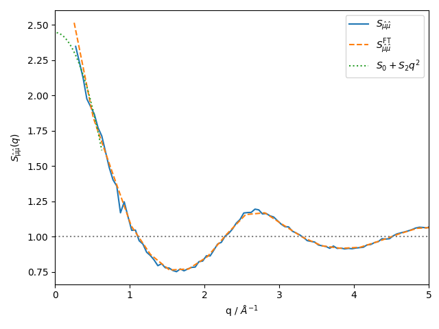
You see that the orange and the blue curve agree. We also add the fit as a green dotted line. From \(S_0\) we can extract the dielectric constant via [7]

\[\frac{\mu^2}{\varepsilon_0} S_0 = \frac{(\varepsilon - 1)(2 \varepsilon + 1)}{\varepsilon}\]

This formula can be inverted and an estimator for \(\varepsilon_S\) can be obtained as we show below.

def dielectric_constant_struc_fact(S_0: float, molecular_dipole_moment: float) -> float:
    """The dielectric constant calculated from the q->0 limit of the structure factor.

    Parameters
    ----------
    q_0_limit : float
        the q -> 0 limit if the dipololar structure factor
    molecular_dipole_moment : float
        dipole moment of a molecule (eÅ)
    """
    dipole_moment_sq = (
        molecular_dipole_moment
        * scipy.constants.angstrom
        * scipy.constants.elementary_charge
    ) ** 2

    S_limit = (
        dipole_moment_sq
        * S_0
        / scipy.constants.epsilon_0
        / scipy.constants.elementary_charge
        / scipy.constants.angstrom**3
    )

    return (np.sqrt((S_limit) ** 2 + 2 * S_limit + 9) + S_limit + 1) / 4


epsilon_struct_fac = dielectric_constant_struc_fact(
    S_0=eps_fit.coef[0], molecular_dipole_moment=dipole_moment
)
print(f"ɛ_S = {epsilon_struct_fac:.2f}")

ɛ_S = 53.53

Which is quite close the value calculated directly from the total dipole fluctuations of the simulations \(\varepsilon_\mathrm{MBE}\approx69\). This difference may result in the very crude fit that is performed and it could be drastically improved by a Bayesian fitting method as for example for fitting the Seebeck coefficient from a similar structure factor [8].

References

[1] (1,2)

Carlos Vega and Jose L. F. Abascal. Simulating water with rigid non-polarizable models: a general perspective. Phys. Chem. Chem. Phys., 13(44):19663–19688, November 2011. doi:10.1039/C1CP22168J.

[2]

Martin Neumann. Dipole moment fluctuation formulas in computer simulations of polar systems. Molecular Physics, 50(4):841–858, November 1983. doi:10.1080/00268978300102721.

[3]

Cui Zhang and Giulia Galli. Dipolar correlations in liquid water. The Journal of Chemical Physics, 141(8):084504, August 2014. doi:10.1063/1.4893638.

[4] (1,2)

Chao Zhang, Jürg Hutter, and Michiel Sprik. Computing the Kirkwood g-Factor by Combining Constant Maxwell Electric Field and Electric Displacement Simulations: Application to the Dielectric Constant of Liquid Water. J. Phys. Chem. Lett., 7(14):2696–2701, July 2016. doi:10.1021/acs.jpclett.6b01127.

[5]

H. Fröhlich. Theory of Dielectrics: Dielectric Constant and Dielectric Loss. Monographs on the Physics and Chemistry of Materials. Oxford University Press, 2 edition, 1958.

[6]

J. M. Caillol. Asymptotic behavior of the pair-correlation function of a polar liquid. The Journal of Chemical Physics, 96(9):7039–7053, May 1992. doi:10.1063/1.462536.

[7]

Jean-Pierre Hansen and Ian. R. McDonald. Theory of Simple Liquids. Elsevier / Academic Press, 3rd ed edition, 2006. ISBN 9780080455075.

[8]

Enrico Drigo and Stefano Baroni. Seebeck Coefficient of Liquid Water from Equilibrium Molecular Dynamics. J. Chem. Theory Comput., 19(23):8855–8860, December 2023. doi:10.1021/acs.jctc.3c00760.